As it happens, water doesn’t compress very much. I would tell you what happens if you jump a hundred feet into the water, but then I would have to kill you. Of course, if you did that, you would already be dead. You know, because water hates you.
Thankfully, files do compress. Compressing files magically makes them smaller. Decompress them later and you get the original contents back.
This is obviously quite useful. Compressed files take up less space on storage devices and less bandwidth when transferred over networks. That is all well and good, but how does file compression actually work?
File Compression
When we compress files, we need to represent the same contents with less information. Thankfully, most files have redundancy. This means that the same data is included in the file more than once, which leaves room for further compression.
Let’s say we have a simple text file:
AAAABBBBCCCCCCCCCCCCCCCCCCCC
This takes up 28 bytes. Still, it isn’t really 28 unique bytes – most of these characters are the same. By noticing that we could come up with another representation:
4A4B20C
In other words, there are 4 A’s, then 4 B’s, then 20 C’s. This is enough information to expand it back into the original file. But we represented it with only 7 bytes, 25% of the original size.
This is a simple example, of course. Most people – excluding present company – have learned their ABC’s already. How about something real?
Suppose I said this:
I put an apple in the fridge. I put cheese in the fridge. There are two things in the fridge.
Our technique before with letters will not work very well here. We need a better solution.
One method is to use a dictionary. This dictionary will not contain the definitions of words. Instead, it will give each redundant word (or group of words) a number. We will make a list of words and then replace them by their numbers in the sentence.
Here is a dictionary:
- I put
- in the fridge
Now our sentence becomes:
1 an apple 2. 1 cheese 2. There are two things 2.
This is much smaller. The original sentence was 93 bytes. The compressed sentence is 49 bytes. Much better, right?
Not quite. The compressed sentence is much smaller, that much is true. But how do we turn the compressed sentence back into the original? We use the dictionary. The dictionary needs to be included in our count because there is no way to decompress the sentence without the dictionary.
When we count the words in the dictionary we get 18 bytes, for a total of 67 bytes. We also need to add the numbers and the spaces in the dictionary because the words alone don’t help us. That adds 4 bytes for a total of 71 bytes. The compressed data is 22 bytes smaller.
This is a good time to introduce the compression ratio. That is, the ratio between the uncompressed size and the compressed size. In this case, the ratio would be 93:71. For every 93 bytes of the original, we end up with 71 bytes when compressed.
Another useful metric is space savings. Space savings is how much we reduced the data size by. For example, if our space savings is 80% it means the size of the compressed data is only 20% of the original. In this case, our space savings is 24% – the compressed data is 24% smaller.
The effectiveness of compression varies based on the method of compression and the data being compressed. For example, the sentence I used here was fairly redundant. This enables it to be compressed fairly well. If I added more items to my fridge, it would compress even better because the redundant parts become a larger percent of the sentence.
In contrast, with a single random sentence the compression would likely be less effective because most sentences don’t contain much redundancy within themselves. The more data you have, the more patterns can be found. You would likely get better compression on this entire article than the first sentence of it.
The method I described above is used for compressing text. It is also the base concept behind the DEFLATE algorithm, which is what is used to make .zip files. Compression is also extremely common in image, audio, and video file formats. This is primarily because these files are quite large in raw format.
Image Compression
Consider an image. Images are composed of many pixels. Here is a 100×100 image:

This image is pretty small compared to most. It has 10,000 pixels.
Each of these pixels is a specific color. Each color is represented as a red, green, and blue value, each a byte. Furthermore, the PNG format supports transparency, which is another byte. Thus, each color is stored as four bytes. This gives us a raw (not PNG) image size of 40,000 bytes, or 40KB. Not so bad.
What if this image was 200×200? That gives us a total size of 160KB.
400×400? 640KB.
600×600? 1.4MB. As you can see, it grows quickly. 1.4MB doesn’t sound like that much, but when you are downloading a web page with multiple pictures it makes for a sluggish experience.
For reference, here is a bigger version at 600×600:

The actual 600×600 PNG, when compressed, weighs in at 615KB. That is pretty good – well under half of the original size.
PNG actually does much better than that, though. PNG has multiple steps of compression that do different things. One of them is to use a palette. Rather than storing the RGB values for each pixel, it stores RGB values for each color in the picture and then each pixel stores the index of that color. This functions much like the dictionary before. As you might imagine, it saves a significant amount of space because a lot of pixels are the same color.
This particular picture is actually one PNG doesn’t work as well for because it has so many colors. When less colors are used the compression becomes even more efficient.
Consider another 600×600 picture. Recall that in a hypothetical raw format, the size of said picture would be 1.4MB. The size of a PNG image at that size with many colors is 615KB.
Look Ma, I am an artist:

Notice that there are only four colors in this picture. It is still 600×600. How big is it?
6KB. Substantially less than both the raw format and the PNG with many colors. It is one-hundredth the size of the other PNG file.
Audio Compression
The approach to compressing audio data is generally twofold. The first approach is to, as with the other examples, find ways to remove redundant data. Typically audio-specific methods of compression do this better than general-purpose compression algorithms (e.g. zip files).
The other form of compression is to remove details from the audio. For example, removing frequencies outside of human hearing range. This also extends to removing sounds which technically can be heard but cannot be distinguished, like changes in your peripheral vision.
The quality of the audio can also be reduced. It can be expressed as the bit rate. The bit rate is how many bits we use to represent the audio over a unit of time, such as per second or per minute. This is controlled by two factors: the level of detail, and the sampling rate.
The level of detail is how much information we store about the audio for a single point in time. For example, with 8-bit audio we can represent 256 different levels of volume. With 16-bit volume we can represent 65,536 different levels of volume. The higher the detail, the closer it represent the “real” sound.
The sampling rate is how often we sample or record the audio information per second. Consider watching a movie. Movies consist of 24 frames per second. When you watch a movie, you aren’t watching a continuous stream of action. Instead, you are watching a series of individual images that, when played fast enough, look continuous.
Audio works the same way. We record a “picture” of the audio many times each second. The number of times we do this per second is the sampling rate. Contemporary audio often uses a sampling rate of 44.1 kHz – 44 thousand times per second.
Here is one of those illustrative diagram thingies:
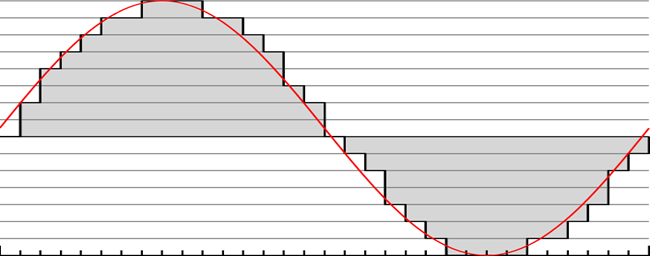
This represents a sound wave. The sound wave itself is the red line. The gray rectangles (they are vertical) are the digital approximation of the amplitude.
The level of detail (more commonly known as the bit depth) is how many different heights the gray rectangles can be. The number of heights is equal to 2^n, where n is the number of bits. This picture features a bit depth of 3 (8 values). This is far too low to represent actual sound, but works well for demonstration purposes.
The sampling rate is represented by how many gray rectangles we can fit into a given space. For example, there are 15 rectangles in the left half of the picture. If we reduced the width of each individual rectangle, we could fit more of them into the same space. Increasing the sampling rate is the same thing as reducing the width of the rectangles.
Notice that there is white space between the top of the rectangles and the red line. The larger the white space the more the recorded audio deviates from the real sound. This deviation is affected by both the bit depth and the sampling rate. If we increased the bit depth, each rectangle could better match the exact height at its location. In the picture, the rectangles both overvalue and undervalue the real sound because they must be on the nearest amplitude line. Similarly, if we increase the sampling rate it allows the smaller rectangles to represent smaller stretches of the wave, and so be more precise.
The bit rate is affected by both the sampling rate and the bit depth. It is the product of these two factors. For example, if we have a bit depth of 16 and a sample rate of 44.1 kHz, the bit rate is 705.6 kbits/second, or 88.2 KB/s (8 bits per byte). This is also the bandwidth that will be used when streaming audio.
Video Compression
If you have ever downloaded a video file, you likely know that they are massive. This makes sense, really: they contain a bunch of images and audio, so they are bigger than any single image or piece of audio.
Video files are, for the most part, largely empty containers. They contain two data sources within them: the video encoding (the images), and the audio encoding. Both the video encoding and the audio encoding could exist by themselves outside the container. The container is just what groups and synchronizes them together. Due to this, the audio encoding in the video file is the same as the audio compression I covered earlier. The focus of this section is on the video encoding formats.
Video is really a series of single images strung together fairly rapidly. Given that, you might guess that video encoding is just a string of compressed pictures – and you would be wrong. Why?
Image compression works well for single images. However, even these compressed images are too big when you add it all up. If we have a five minute video that has 30 frames per second, that is a total of 30*60*5, or 9,000 frames. Our best-case PNG image was 6KB. Repeating this image every frame would add up to 54MB. In contrast, our worst-case picture was 615KB. That would bring us to 5.5GB.
Still, those are edge cases. Let’s pick in the middle and go with 100KB. I choose that because the worse-case picture would be better off as a JPEG. 100KB, on the other hand, is quite plausible. That adds up to 900MB. That simply will not do.
What can we do about this? Recall from earlier that compression tries to minimize redundant data. As it happens, videos have a lot of redundant data. Consider a video of a politician speaking. The politician moves frequently and is in motion most of the time. What about the background? It doesn’t change. It is redundant.
Think of a video as a stream of pictures. Each picture will contain the same background. That is wasting a lot of data because the background doesn’t change.
Imagine playing a video as stacking these pictures on top of each other. What if we cut out the background of every image but the first one? It would still look the same, because the background from the first layer is carried forward in every later picture. The parts we cut out our redundant. This is exactly how video compression works. Rather than a series of images, it is a series of changes to the original image. This uses significantly less data.
For compression purposes, video frames are considered in terms of macroblocks. A macroblock is an 8×8 block of pixels. You can imagine it like a grid overlaying an image.

Each frame, a command is given for each of these macroblocks. For example, if a macroblock is in the background, the command will be to do nothing. If the macroblock is part of the politician, then it will be an update command containing what pixels changed. There are also more complex commands, like moving a macroblock by a certain offset (picture a moving square), rotating it, changing the colors in it, and so on. There are also commands for interpolation, which is a fancy word for “guess what color this is based on what is around it.”
Thus, video encoding stores changes over time. This is vastly more efficient. If you look at most videos, you will notice a lot of redundant data that stays the same for a while. It doesn’t need to stay the same for long, even – a background that lasts for a second can still be compressed. You will also note that videos can still contain anything – they don’t need to have the same background throughout the entire video, for example.
The compression ratio for video files is massive, absolutely massive. And it has to be. If it wasn’t, video streaming wouldn’t exist at all because the amount of data contained in videos is far too large to send over the internet. Thankfully, video compression methods are quite effective and they make video streaming very possible.
As with audio, video has a bit rate. The commands given to the macroblocks require a certain number of bits. The higher the bit rate, the more commands can be given per second. Conversely, a low bit rate will mean fewer commands can be given per second. When many commands can be given, more of them are used for tiny detail changes. When there are fewer commands available, smaller details may be left unchanged and slightly messed up. Thus, the bit rate is effectively a measure of video quality. As before, it also serves as a measure of bandwidth.
Lossy And Lossless Compression
All compression methods can be divided into two camps: those that are lossy, and those that are lossless. What does that mean?
Lossless compression doesn’t lose any information. Given the compressed data, you can perfectly reconstruct the original exactly as it was before.
Lossy compression, as the name implies, loses stuff. Once you use a lossy method of compression, you cannot get the original data back anymore. Lossy compression usually “tosses out” details that aren’t readily noticed. For example, in an image exact color reproduction isn’t particularly important: the human eye does not notice such things. Due to this, certain areas of a picture may all become the same color when compressed, thus requiring less data.
Lossy compression allows much smaller file sizes because it doesn’t need to include all the data – this is the primary reason lossy formats are used. Generally speaking, significant size reductions are possible with lossy compression (10:1 or so), while the difference in quality is hard to perceive. Lossless compression, on the other hand, will yield relatively larger files because it must retain all the information. The result of this trade-off is that files with lossless compression always stays the same quality, which cannot be said for lossy formats.
There are plenty of compression methods in both camps. For example, PNG is lossless and JPEG is lossy. MP3 is lossy and FLAC is lossless. The list goes on.
Generally speaking, content in its original, high-quality form – a photographer’s picture, a video being edited, a song that was recorded, and so on – is stored in a lossless format so all the information is kept. It is only when it is later distributed that its form will change. For example, suppose there is an original high-quality image file. A resized version of it may be used to print in a magazine, and a compressed JPEG version may be available on a website. The JPEG version wouldn’t be good enough to use for printing, but its small filesize is very beneficial on the web. In effect, there is a “master” source file.
Interestingly, this is also why bluray movies look better than DVDs. The original movie is stored in very high quality. However, DVDs can only hold 4.7 GB. To make it fit, the movie is resized and compressed using a lossy format. This degrades the quality, but allows the movie to be distributed. Blurays, however, can hold 25GB. Thus, they can create a new version from the master file that is much higher quality than the DVD. The result is a sharp increase in quality.
There are a few general guidelines for changing the format of a file. Going from a lossless format to a lossless format is always perfect. Going from a lossless format to a lossy format loses information, but gives the benefits that come with a smaller file size. In contrast, you want to avoid ever changing from a lossy format to any other format – lossless or lossy. If you go from lossy to lossless, you don’t gain any more quality, but increase the filesize. If you go from lossy to lossy, you lose even more information. As a general rule, if you want to make different lossy versions, you should make them all from the master lossless file.
Usually lossy format files still look fine. Still, if you know what to look for you can see evidence of the changes. Let’s take a look with this cat:

Nice little kitty. Let’s zoom in.

Pixely, of course, but something else isn’t quite right here.

See those blotchy areas around the whisker? That is a compression artifact. This is where detail was thrown away. You couldn’t see it in the full size image, but you can here. When images are heavily compressed or compressed repeatedly (for example, editing an image somebody else uploaded) with a lossy format, these artifacts worsen. Eventually they are visible at normal size.